Introduction
Most of the time, we decide facing a certain degree of uncertainty. This is often due to the fact that not only we have several options but we also are unable to correctly predict how they are going to affect our situation.
In these cases, we tend to act according to a subconscious evaluation of the probabilities associated with each scenario. Yet, we do not seem surprised to turn to diversification the moment we desire to smooth out such uncertainty. Indeed, it does not only make sense practically but seems to point directly to what a sound decision-making strategy should look like in the real world.
Diversification, on its side, appears to be an ancient – yet incredibly modern – idea. Indeed, it has not only influenced modern sociology, evolutionary theory, and genetics but has also served to shed light on a non-trivial aspect of human behavior: the preference of variety over uniformity when the outcomes are uncertain.
This is especially true in the world of investments. In this sense, diversification forms the cornerstone of financial decision-making to the extent that an imaginary line could be drawn from the Modern Portfolio Theory developed by Harry Markowitz in the early 1950s – that highlighted the role of correlations as the driver of diversification – to a Talmudic quote dated ca. 600 AD in which we find the first allusion to what in Finance is known as asset class diversification:
“It is advisable for one that he shall divide his money into three parts, one of which he shall invest in real estate, one of which in business, and the third part to remain always in his hands.”
Yet, as one could imagine, although it is simple to grasp its benefits, diversification does not come off easily. Indeed, it becomes a rather complex task to achieve when financial markets change, become faster and the dynamics between assets and asset classes move continuously to reflect the underlying unfolding of the economic cycle.
For this reason, we can expect diversification to evolve as well – from a well-known principle to a more precise, measurable and quantitative risk management strategy – to reflect on the one hand the most recent technological advances and, on the other hand, to leverage data to have a better understanding of the real risks our portfolio is exposed to and make it work in the long term.
Start integrating AI into your investment process with the most advanced no-code solution.
Book A Custom Demo
The E=MC2 of Finance
It was 1905 when Albert Einstein published his famous article on the symmetries of space and time entitled “Does the inertia of a body depend upon its energy content?”. In his paper – that went down to history as the origin of the famous equation E=mc2 – appeared for the first time an explanation of what is called in Physics the mass-energy equivalence, meaning that anything having mass has an equivalent amount of energy and vice versa. Apart from the apparent simplicity of the equation, what was set to be paradigm-shifting about Einstein’s contribution was that it radically changed the way we saw nature, establishing a link between quantities (i.e. energy and mass) that had eluded scientists for centuries.
To a certain extent, Finance lived a similar breakthrough approximately 50 years later. In 1952, Harry Markowitz published “Portfolio Selection”, the paper in which he put together the three elements of investing – risk, return and correlations – to form a consistent framework for portfolio construction and diversification.
At first sight, his advice was fairly straightforward: “don’t put all your eggs in one basket”. With that, he hinted at the fact that, ideally, there is less risk in holding a portfolio made up of many securities rather than concentrated bets that might eventually not pay off as expected. As a result of this, diversification – the reduction of risk achieved by spreading investments – became how the same return could be achieved with a lower level of risk. Markowitz’s legacy is indeed closely tied to having changed the way asset and investment managers saw investment decisions under uncertainty, as he exposed the mechanism that allowed the balancing out of gains and losses: the correlations between securities in the portfolio.
He showed that in order to achieve diversification, what was needed was not a great number of assets (as a naive strategy would have required) but rather selecting securities according to their relative correlations. Indeed, what appeared sufficient was to choose a set of decorrelated (or negatively correlated) positions so that, on average, their comovements would balance out and reduce the overall volatility of the portfolio.
Eventually, his contribution advocated for a radical change in the way portfolios were managed. Efficiency (i.e. the ratio between risk and return) became what investors had to look for in their investments and diversification what allowed it to happen. Indeed, as a result of the introduction of a quantitative model to allocate among securities, the benefit of diversification could finally be objectively measured rather than being based on a qualitative judgment.
The More The Merrier? Not Always
So far, the lesson we learned is that diversification comes as the result of how securities move among each other instead of how many assets are included in the portfolio. In order to achieve it, securities need to move together the least possible so that the gains on some investments can outweigh the negative performance of others.
In this light, we understand the role of correlations in this process: they measure synthetically (i.e. in a range from -1 to +1) the direction of how assets move with respect to each other. A positive correlation indicates that assets tend to rise together and fall together while, on the contrary, a negative correlation means that assets tend to move in opposite directions, thus balancing out. In between the two, decorrelated assets (i.e. the ones that exhibit almost null correlation) tend to move independently from each other.
With this in mind, it becomes clear why assets that are low or negatively correlated represent the key to achieve diversification. For instance, we can imagine choosing among three hypothetical assets with the following ex-ante expected return and volatility, shown in Exhibit 1.

We can form two equal-weight portfolios made up of the three assets and compare their expected return, volatility and efficiency in two scenarios: high correlation (i.e. with an average correlation of 0.8) and low correlation (i.e. with an average correlation of 0.2).

What we get from this example is that diversification not only is about risk-management but also helps to achieve more efficient use of capital. Indeed, Exhibit 2 shows the benefit of choosing assets that exhibit low average correlation.
Even though Portfolio A and Portfolio B share the same expected returns, there is no doubt that an investor would like to hold the latter (that has an average correlation of 0.2) as it has almost 20% less volatility and about 30% more risk-adjusted return (i.e. efficiency).
Measuring the Diversification Benefit
Eventually, what we have seen until now is the stepping stone to ask another question: what is the marginal benefit of diversification?, or alternatively, how much risk can diversification take away?
So we can imagine carrying out another experiment: we start with a portfolio of only one asset, which has a volatility of 10% and an expected return of 5%. Then we add more assets with equal risk-return profiles to create an equal-weight portfolio. Eventually, we calculate the overall volatility of the portfolio and plot it. We repeat this process up to 15 assets and then repeat the whole experiment for different levels of average correlation. Eventually, we will see a plot similar to the one shown in Exhibit 3.

In Exhibit 3 we see the level of diversification benefit – the reduction in portfolio volatility that occurs as we add more assets into the portfolio – for different levels of average correlation. As expected, the first thing we notice is that in each portfolio, the volatility (measured on the y-axis) is reduced as soon as we add more assets (measured on the x-axis) for every level of correlation.
However, what appears to be insightful here is that the amount of the reduction is an inverse function of the average correlation between the number of assets, that is, it increases as the level of correlation gets lower.
Indeed, we see that even if we add many assets with a high average correlation (i.e. the blue line), the reduction achieved is less than 1%. Conversely, if we keep adding to our portfolio assets that have low correlation or are totally decorrelated, the diversification benefit grows larger and eventually gets as high as 80%. This means that from the initial 10% of volatility, we reduce it to about 2%, with an increase in the initial risk-return ratio by a factor of 5.
Opportunities Lie Between and Within Asset Classes
Until now, we have introduced diversification as the main strategy an investor can use to reduce the investment risk. Indeed, guided by intuition, we have understood that the key to a well-diversified portfolio lies in the structure of its correlations and eventually we have been able to measure its benefits and quantify what it means to add value to a portfolio in terms of efficiency.
Diversification has eventually revealed itself under a new light, escaping a simplistic or vague explanation, in favor of a more precise and actionable definition of diversification benefit. Indeed, it has provided on the one hand an objective criterion to select and weigh investment ideas and, on the other hand, it has emerged as a multidimensional process that needs to be integral in every stage of portfolio construction.
As a matter of fact, many times asset and investment managers find themselves building their portfolios according to a hierarchical process. This means they initially set the percentage of the portfolio to be allocated in each asset class, (e.g. stocks, bonds, liquidity) and then proceed to choose which securities to invest in accordingly. In this sense, we get why diversification is multidimensional: because it can be achieved both at an asset allocation level (i.e. diversification between asset class) as well as at the more granular security selection level (i.e. diversification within instruments in the same asset class).
However, in practical terms it all boils down to the nontrivial question of what can be considered as a diversifying opportunity. Indeed, it appears that we first need a way to measure the current level of diversification and, from this standpoint, determine if a candidate investment is an opportunity or not on the basis of how much benefit it adds. In particular, as diversification has to do with volatility, we can imagine such a measure to establish a connection between two quantities: the volatility of the single investments and the volatility of the current portfolio. One example can help show how this process can be put into practice.
Imagine we hold an equal-weight portfolio with an average correlation of 0.8, as we did with Portfolio A in Exhibit 1. A quick way to calculate how much this portfolio is diversified is obtained by determining its diversification ratio (DR), that is, the ratio of its weighted average volatility to the portfolio volatility.
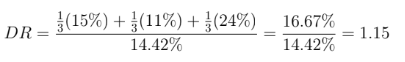
This ratio tells us an important piece of information about our current portfolio. It helps us understand how much the correlations between the three assets lead to a reduction in volatility (i.e. 15% less), compared to taking separate bets on each security.
We can also use the diversification ratio to assess if a candidate investment opportunity can be also considered a diversifying opportunity, as we initially desired.
Indeed, we can expect the marginal contribution to diversification given by each addition to the portfolio mix to be a fundamental piece of information that an asset or investment manager wants to know during his or her decision-making process. This helps us think more clearly about what a diversifying opportunity really is: it is a change in the portfolio composition that improves the current level of diversification.
In our example, if we assume the diversification ratio to be a good proxy of the current level of diversification, a diversifying opportunity would be a candidate investment that – once added to the portfolio – makes the diversification ratio grow larger than 1.15 (i.e. that increases the spread between the weighted average volatility and the volatility of the portfolio). Indeed, from a diversification standpoint, a portfolio with a diversification ratio higher than this threshold would be preferable.
However, it seems that when we look at diversification only from a static and uniperiodal point of view, we miss something that is a typical trait of real-world investing, that is, that diversification is not going to last forever. Indeed, even a well-diversified portfolio will eventually incur a change in its degree of diversification with the passage of time and will need to be periodically updated and rebalanced to better reflect new opportunities available in the market.
This is due to the fact that financial markets not only are complex environments but also change continuously. As a result of this, the relationships between assets and asset classes evolve and so do their correlations that capture synthetically this piece of information. Eventually, we understand that diversification must evolve to accommodate the economic cycle that unfolds gradually and, as we are going to see, a more granular sector- and factor-based approach becomes essential to meet it on an ongoing basis.
Why Sectors Matter
Imagine that we have decided our asset allocation and find ourselves in a situation similar to the one represented in Exhibit 4. We may be confident that this mix achieves a good level of diversification and so we proceed to select some broad and liquid securities that can represent each asset class in our portfolio accordingly. For example, we choose an ETF on the S&P 500 for Equity. Again, we look at our portfolio and ask ourselves, is it diversified enough?

If we look deeper at the Equity portion and break down its actual allocation, what appears is that our portfolio reflects an implied allocation in sectors that we are not able to control. Indeed, this choice is inherited from the underlying benchmark which weights companies according to their relative market capitalization (i.e. in the S&P 500 larger companies by market capitalization weight more than small companies). For example, Exhibit 5 shows the current sector allocation of the S&P 500 Index.

What we see is that eventually, almost 50% of our equity risk is linked to the performance of 3 sectors, namely Information Technology, Health Care and Financials. Is that what we originally desired? and moreover, is this sector allocation well-diversified?.
It seems that unless we believe this composition reflects our risk-return preferences, we should care a great deal about sectors, in the sense that they reflect another point of view on the real risk exposure of our equity portfolio. Besides, it feels reasonable to assume that diversifying between them is going to add value just as much as it did with asset classes in the previous examples.
Specifically, sectors refer to a classification used to describe companies that belong to the same segment of the economy (e.g. Utilities, Real Estate, Oil & Gas). In particular, even though there are slightly different classifications across geographies or data providers, when asset and investment managers talk about sectors they usually refer to the 11 GICS Sectors (i.e. Global Industry Classification Standards), namely:
- Energy
- Communication Services
- Materials
- Industrials
- Consumer Discretionary
- Consumer Staples
- Health Care
- Financials
- Information Technology
- Utilities
- Real Estate
At first sight, the reason why they exist appears to be straightforward. Indeed, as they group companies according to the nature of their business, they allow us to monitor independently different corners of the market and have a more granular representation of the underlying economy.
Besides, since we can imagine each one of them to respond to sector-specific dynamics (e.g. companies in the industrial sector could be more sensitive to shocks in the price of oil), sector classification is also a useful risk management tool to assess and better calibrate the risk exposures of our portfolio. From this standpoint, diversifying the equity portion of the portfolio also across sectors appears an interesting strategy to follow.
Indeed, as a result of being driven by different sources of risk, sectors exhibit a great dispersion in correlation among one another and so they represent a chance to add an extra layer of diversification by allocating to market segments that are uncorrelated among each other.
We can see this by looking at Exhibit 6, which shows the three-year correlation matrix between the sectors of the S&P 500 Index. This matrix gives a clear picture of how correlations among sectors work and gives also an initial indication about where the opportunities of diversification lie.
As expected, we see immediately from its analysis (i.e. in which colors reflect the intensity of correlation) that not all sectors move in sync with one other, but instead they tend to form clusters. This gives us a great piece of information that we can use to determine sector allocation, that is, that opportunities lie between the different clusters.
Indeed, one should avoid too much concentration in highly-correlated sectors that belong to the same cluster (i.e. the Technology, Consumer Discretionary and Health Care sectors have an average correlation of 0.75) but instead mix them with sectors that tend to decorrelate sharply from the other ones (i.e. as it happens for Utilities, Consumer Staples and Real Estate sectors) to add an additional layer of diversification to the portfolio.

Diversification Benefit: Sector vs Market Cap
In order to have a better insight into the diversifying opportunities offered by sectors, we can perform the following analysis.
We initially divide companies according to market capitalization (i.e. small, mid, and large cap) and by sectors. Then, we compare and sort the diversification benefit achieved by two sets of equal-weight strategies: the first one diversifies across market capitalizations but invests in one sector only; the second one equally weights across sectors, while investing in one segment of market cap at a time.
Indeed, the component we are trying to isolate here is relative to the benefit of choosing sectors (instead of capitalization) as diversification criteria.
As a matter of fact, since they exhibit a much wider set of correlations to choose from, we expect the diversification benefit achieved by spreading money across sectors to be higher with respect to market capitalization.
In Exhibit 7 we see the results of this analysis, in which - for each strategy - the portfolios have been sorted according to their degree of diversification benefit.
As expected, we see that the strategies that diversify across sectors and hold market capitalizations constant are able to attain a much higher diversification benefit – in the magnitude of four times – when compared to the strategies that invest according to market capitalization.

Not All Sectors Are Born Equal
As mentioned, the reason sectors are different is because they represent different business activities. In this sense, we have no difficulty in believing that there are intrinsic characteristics that make, ideally, companies that belong to the financial sector (e.g. banks, insurance companies) more sensitive to changes in interest rates with respect to communication or health-care companies. Alternatively, it seems also reasonable to believe that technology-intensive firms can experience more rapid (or even exponential) rises and falls with respect to, for example, a utility company. Eventually, sectors not only are a matter of mere classification, but also reflect – on aggregate – structural differences in both the fundamentals of such companies (i.e their main balance sheets items) as well as in their business models.
For this reason, some sectors tend to go in the same direction or go against the underlying economic cycle (i.e. be pro or countercyclical), that is, to exhibit positive or negative correlation with it.
Moreover, apart from the economic rationale, what appears to be insightful to better understand sectors is their exposure to known risk factors. As a matter of fact, since the companies that belong to a specific business face different risks, each sector expresses a unique composition of risk premia – sources of uncertainty that financial markets reward with an additional compensation. That is the reason why when we allocate to sectors, we also want to know which risk factors we are exposing ourselves to.
Risk factors are an additional piece of the puzzle to explain why sectors tend to perform differently. In this sense, we can take the five most known factors (Market, Size, Value, Investment and Profitability) – also known as the Fama-French Factors – and calculate how much sectors are exposed to each one of them. In this sense, as the charts in the next page show, we can take a group of eleven sectorial ETFs and explain their returns in terms of factor exposures to see how this has evolved over the last 10 years.
By looking at Exhibit 8, we have the opportunity to expand the initial intuition we had when looking at the previous correlation matrix. Indeed, it seems that the most correlated sectors are also the ones in which the degree of exposure to the underlying market is higher and vice versa.
Besides, although it seems that factor exposure is not constant, for some sectors it tends to be more consistent over time, suggesting that also the signal-to-noise ratio is different across sectors. Thus, we understand that decomposing the sector-specific performance into risk factors is an essential part of understanding the sources of uncertainty each sector is exposed to as well as to identify the real risks of our portfolio. Eventually, it helps to look at diversification from a different angle: in order to achieve effective diversification, one should look at it in its many dimensions, and avoid having a high concentration on the same factor.

Where do we go from here?
As financial markets change and become more complex environments, knowing only why diversification happens and why it is beneficial seems insufficient to keep risk under control. On the contrary, in recent years the focus has incrementally shifted on its how, that is, expanding and refining the traditional toolbox to identify new opportunities and achieve it on an ongoing basis.
From this standpoint, what asset and investment managers face today is a twofold challenge. On the one hand, diversification has emerged as a multi-period and multidimensional protocol that needs to be taken into account during all stages of the investment process: at the asset allocation as well as at the security selection level. On the other hand, a better understanding of the drivers of diversification has led to the development of a quantitative approach to manage risk and to select and benefit-weigh investment ideas according to their added value.
At a deeper level, this challenge marks the transition (or the evolution) from a principle-based to a data and opportunity-driven diversification. In this sense nowadays, lacking a well thought out sector allocation strategy seems a lost opportunity to add an additional layer of diversification, for several reasons.
Sectors represent great diversifiers because of their targeted focus on specific corners of the broad economy, providing a more granular and controlled risk exposure. As a matter of fact, since they are driven by different sources of uncertainty, they also allow expanding the dimensions in which the portfolio can be considered diversified.
Besides, their use appears to be strategic for another reason: their different degrees of sensitivity to known risk premia, hinting at the existence of a double thread between sectors and risk factors. Eventually, this novel opportunity set – which includes sectors and risk factors – opens up the doors to a new approach to diversification, oriented at generating value and better managing the risk-return profile of the portfolio.