Just as we look at fuel economy when we plan on buying a new car, we are used to looking at the Sharpe – the risk-reward ratio – of our investments to see if we are allocating capital efficiently or if we take too much risk compared to the return. Although efficiency is definitely a desirable feature, achieving it takes much more effort than investing in the portfolio that had the best Sharpe ratio in the past. The reason for this is twofold: you cannot invest in the same market twice and Sharpe ratios often lie.
Nevertheless, portfolio optimization is one of the most powerful tools we have to manage investments. Here, we are going to take a closer look at its mechanisms: how it works, why it is useful and which errors we must avoid to do it properly. As we are going to see, it is forward – rather than past – efficiency that we should aim to maximise. To achieve it, we must stop looking in the rearview mirror and position ourselves for stability and efficient market dynamics. In a sense, getting sharper than Sharpe.
You Cannot Invest in the Same Market Twice
Several of the most important ideas of our modern world originated long ago. Especially when it comes to fields that share a centuries-old tradition, such as philosophy, mathematics or astrology, many groundbreaking ideas have been born out of a simple and sometimes naive observation of nature.
In this sense, a big share of those comes from the Ancient Greeks that, from Aristotle to Eratosthenes – the first man able to calculate the Earth circumference almost perfectly in 246 BC – have later revealed the keys to understand the world we live in.
However, it would sound unusual to think that those early philosophers and scientists left an important piece of advice very useful for the modern-day investor. Heraclitus, one of the most influential Greek philosophers known for his sharp wit and keen observations, condensed it into one sentence: “No man ever steps in the same river twice”.
This idea – also known under the famous aphorism pánta rheî – shed light on a nontrivial aspect of our daily life suggesting that rather than remaining still, everything is subject to change and evolve over time. Indeed, even if we do not perceive it immediately, everything flows and mutates from what we initially observed or experienced.
The advice he offered to us is that instead of sticking with a static interpretation of reality we must be ready to embrace the complexity and follow it dynamically. This idea seems to be largely applicable to the world of investing. Financial markets represent a perfect example of a fast-paced and complex environment that slowly changes over time, to the extent that one could say that “you cannot invest in the same market twice”.
We can use this advice to look at financial markets in a new light, and derive two precious insights from it. The first one is that we must look at our decision in terms of investments not as point-in-time but rather as multiperiodal. The second is that every decision we make – even the ones we consider optimal – will need to be updated periodically to reflect the different market conditions that have unfolded in the meantime.
From this standpoint, it is clear why during the last decades portfolio optimization has gained much popularity among asset and investment managers. As the branch of portfolio management involved with finding out which portfolios are optimal under a given set of assumptions, it allows us to have a very powerful tool to navigate and decode the underlying dynamics of financial markets. However, as with any other powerful tool, we must handle it with care and expertise so we do not fall prey to the potential sources of bias that may alter the quality of our results.
As we are going to see, knowing which mistakes need to be avoided is crucial to ensure that the optimization process is done correctly and adds value. To a certain extent, we must be careful about what we wish for, because optimality may not always be a synonym for performance.
Start integrating AI into your investment process with the most advanced no-code solution.
Book A Custom Demo
What is an Optimal Portfolio?
As long as financial markets have existed, investors have looked for a reliable way to allocate wealth efficiently across securities – a mechanism to build portfolios according to their investment objectives.
In this sense, the problem appeared to be twofold: firstly, it was about defining what was meant by “optimal portfolio” and secondly, what process and information was needed to determine it systematically.
It was not until the quantitative approach to portfolio management began to be widespread, that a consensus was reached. Indeed, in the absence of a consistent framework for portfolio decisions, judging if a portfolio was optimal or not was a fairly discretional task instead of something rational and scientific.
Portfolio Management as we know it was born thanks to the efforts undertaken by the mathematician and Nobel-prize winner Harry Markowitz who, in 1952, proposed the first analytical framework for portfolio decisions. His theory – later known under the name of Modern Portfolio Theory – quickly became the industry standard and a cornerstone of modern investing.
Indeed, its success lies in the fact that the model provided asset and investment managers a repeatable process to determine the optimal portfolio using as inputs the information provided by three key variables: the level of risk tolerance, the expected return on each security, and their correlations among each other. Most notably, the latter was crucial to achieve diversification, the degree by which the risk of a portfolio is lower with respect to single bets on each security.
In this sense, the model allowed us to determine which portfolio was best, given a set of initial conditions. This was achieved through a technique called constrained optimization, that is, by finding all the portfolios that either minimised risk for each level of expected return or, the other way around, maximised expected return for each level of risk.
What followed was that – when considered all together – the portfolios that satisfied such conditions formed a line called “the efficient frontier”, as represented by Exhibit 1.
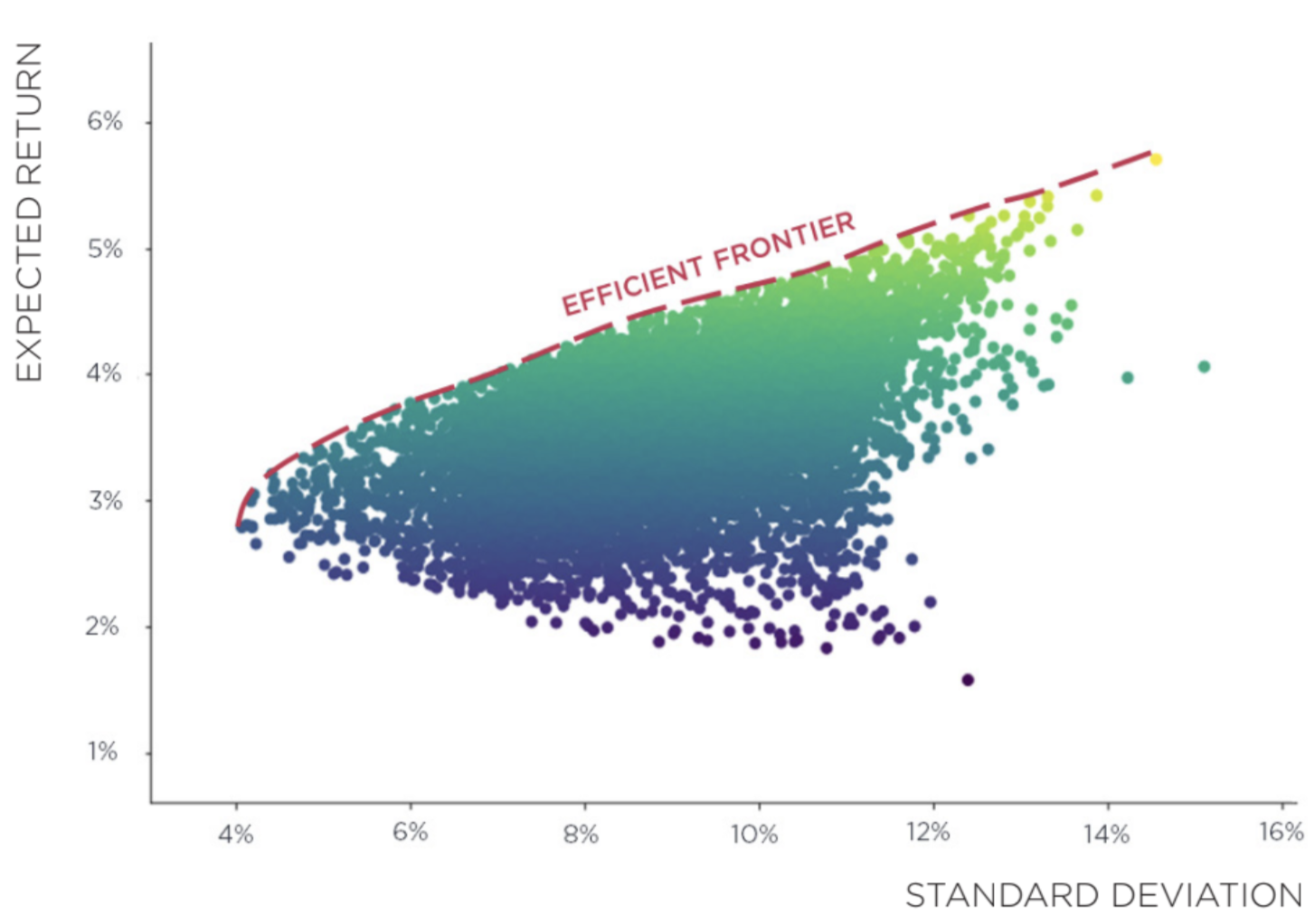
The cloud of points that we see in the graph shows the set of all possible portfolios that can be constructed from the given set of securities, each one represented by its expected return and standard deviation.
In particular, Markowitz advised investors to look only at the portfolios lying on the efficient frontier (i.e. represented by the dashed red line) because they maximize the tradeoff between return and risk.
Among these, each investor will select the portfolio that better suits his risk profile: if the goal is to achieve a portfolio with low volatility - i.e. the investor is risk-averse - then he will focus on the ones lying in the lower left part of the efficient frontier. Conversely, as his level of risk tolerance increases, the investor will take on some more risk in order to achieve higher expected returns, holding portfolios on the upper portion of the efficient frontier.
Optimization is a Moving Bullseye
Under this light, portfolio optimization presents itself as a very powerful tool. Indeed, with the increasing availability of data and computing power, this technique has become increasingly popular in the industry to support asset managers in their investment decision-making. In this sense, from its first introduction in the early 1950s, there have been numerous refinements and adjustments to overcome the limitations that the model posed originally. Indeed, the biggest efforts have been made to adapt this framework to reflect more closely the actual dynamics of financial markets, such as the availability of short selling, leverage constraints, and trading costs, or to minimize the estimation error of the model parameters.
However, as with any powerful tool, it must be managed with care and great expertise. This is because we cannot expect portfolio optimization – as with any other statistical technique – to generate value effortlessly. Instead, these techniques become useful allies only when they are properly understood, managed, and controlled to get the best out of them.
Eventually, it becomes clear how knowing the ins and outs of portfolio optimization is of vital importance: it allows us to reap its benefits while limiting the shortcomings associated with improper use. Specifically, there have been two major areas to receive a lot of attention from both researchers and practitioners in recent years.
On the one hand, a wide literature has focused on investigating the stability of the optimization process with respect to estimation errors in the model’s parameters. Indeed, as expected returns, volatilities and correlations have to be estimated from historical data, estimation errors may bias significantly the final portfolio achieved, resulting in a sharp over or underweight of a security or an excessive turnover.
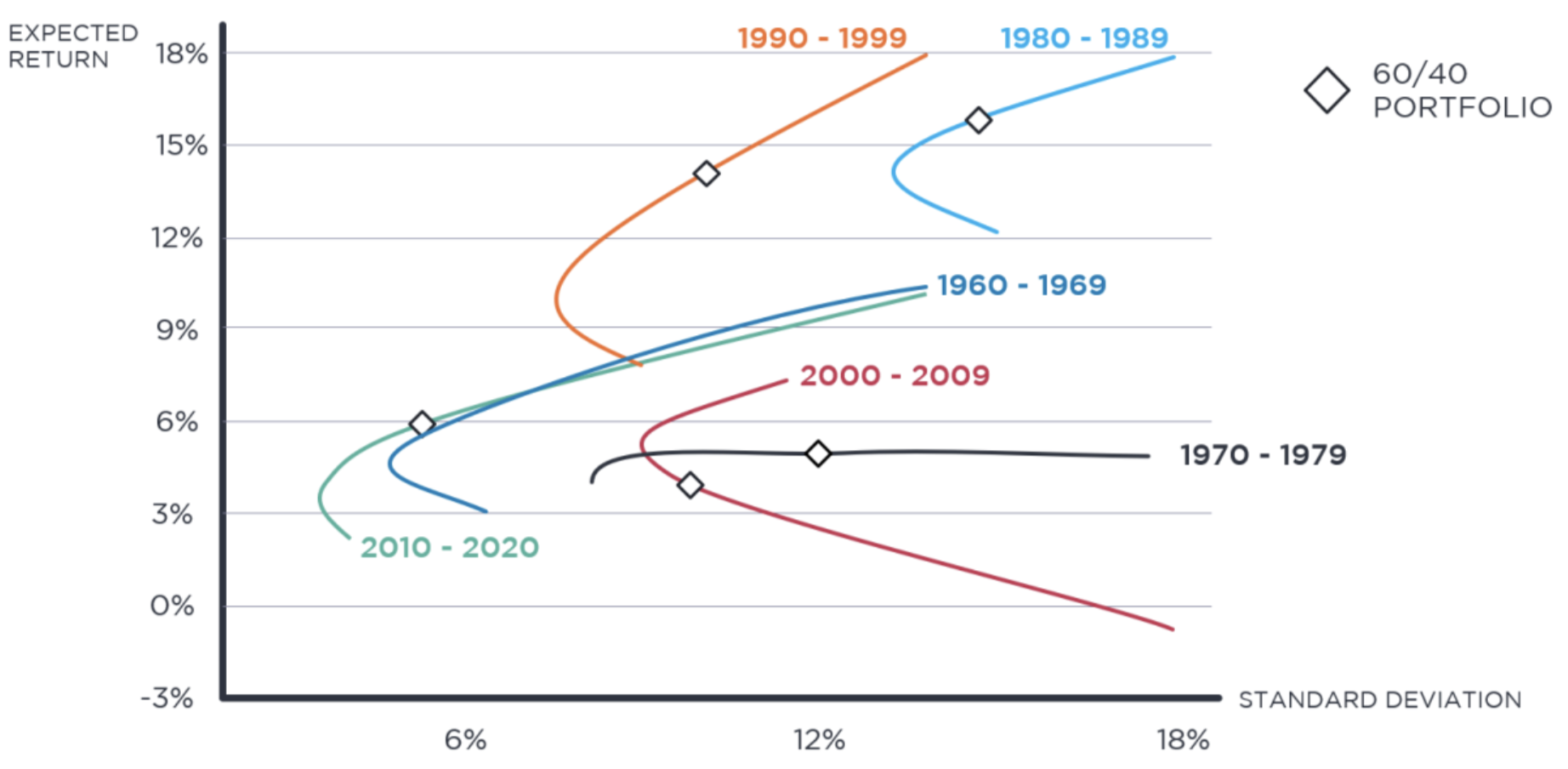
On the other hand, researchers have explored the link between efficient portfolios and their out-of-sample performance, that is, how they perform once they are invested in real market scenarios. In this sense, this area has delivered many precious insights to understand how portfolio optimization can add value in the long term. Indeed, we can expect that as financial markets evolve over time, so does their underlying structure in terms of expected returns, volatilities and correlations between asset classes. This brings up an important remark: instead of being static, the efficient frontier is a moving target constantly reflecting the new market conditions that have unfolded in the meantime, as we can see from the following Exhibit.
Exhibit 2 considers the case of how the risk profile associated with a 60/40 portfolio (i.e. a portfolio invested 60% in fixed income and 40% in equity) would have changed over about 60 years of financial markets, from the 1960s to 2019. As we can see, not only the efficient frontiers move sharply from one decade to the other, but the same asset allocation has completely different risk profiles.
Be Wary of the Efficiency You Wish For, You'll Probably Get It
Starting from its historical developments, we looked at how optimization works and not only described why diversification is of paramount importance during this process, but also explored the pros and the cons of such approaches.
Yet, once we get that applying this methodology adds value to our portfolios, we are left with two additional questions: what is the efficiency we wish for? and can we rely on it?
To a certain extent, it is similar to knowing how a car is built, but ignoring how to drive it. Similarly, even though portfolio optimization is a powerful way to build and manage investment portfolios, it is up to us to decide how to use it to reach our investment goals.
To this point, it is useful to remember what efficiency is about, that is, the ratio between the return and the risk of our investments.
However, as there exist several ways to estimate those two components, we do not have just one way to look at efficiency as a whole, but rather a very broad set of indicators describing the efficiency with respect to a specific aspect of investment risk.
In this sense, the most used indicator for measuring efficiency is the Sharpe ratio – named after the Nobel-prize winner William Sharpe – that compares the expected return in excess of the risk-free rate with the standard deviation of a security over a given time interval, calculated using the following formula:
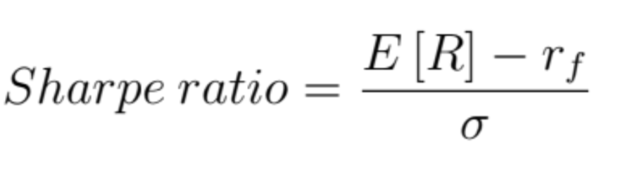
E[R] stands for the expected return of the portfolio, for the standard deviation of its returns and rf for the risk-free rate. In other words, it tells us how many “units” of excess returns we expect to gain from each unit of volatility, measured as how much returns vary over time.
For example, if we consider two portfolios, one that generates a 10% return with a 1.25 Sharpe ratio and a second one that achieves 10% return with a 1.00 Sharpe ratio, the first would be better because it achieves the same return with less risk.
Thanks to its simplicity and ease of interpretation, the ratio has become an important tool in the portfolio management industry. However, it has also been subjected to numerous criticisms coming from both the industry and the academic side – including William Sharpe himself.
These scenarios point to the danger of blindly relying on any single measure for assessing how optimal a specific investment is. For example, we could ask ourselves: what would have happened if we had always invested in the portfolio with the highest Sharpe ratio?
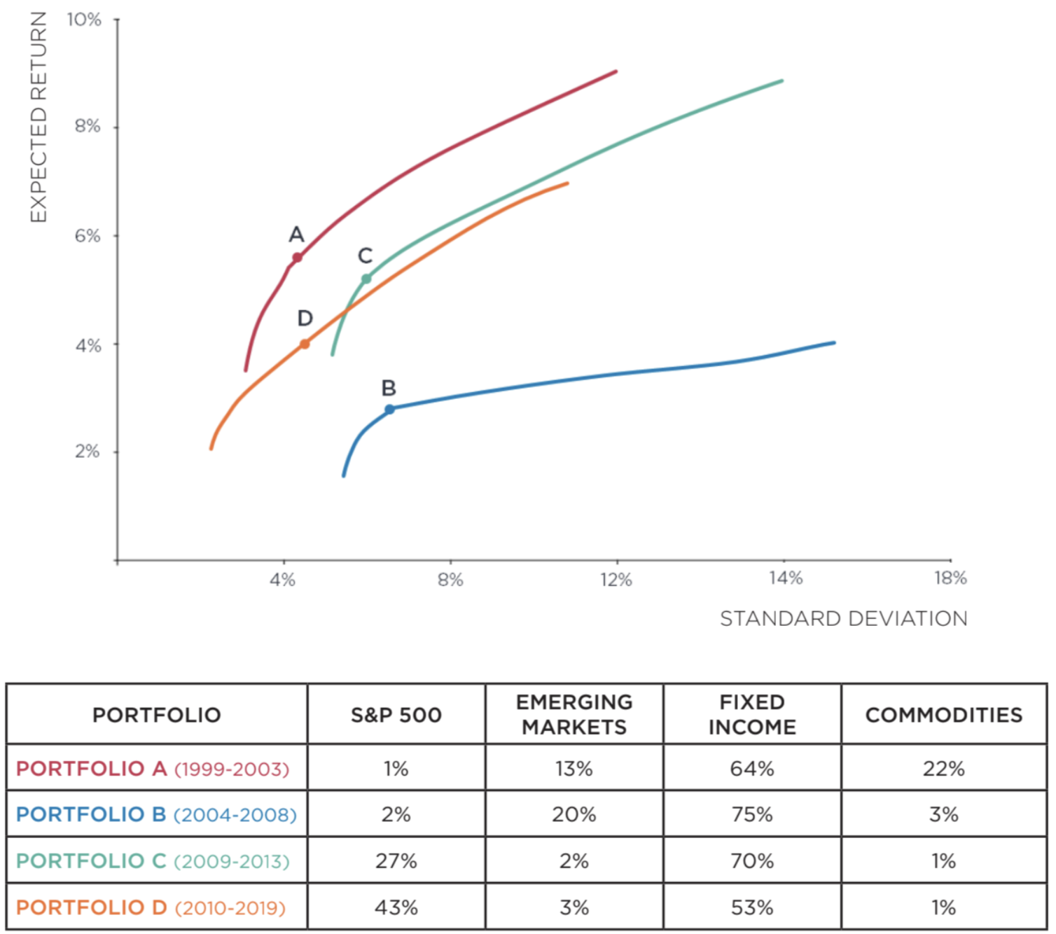
Exhibit 3 shows the efficient frontiers obtained by repeating the portfolio optimization process over 5-years time intervals from January 1999 to December 2019, and the asset allocation of the portfolio with maximum Sharpe ratio. We can immediately see that, as we change the timeframe of our analysis, the efficient frontier sensibly shifts, and so does the position of the portfolio that achieves the maximum Sharpe ratio
When Sharpe Ratios Lie
In addition to the shortcomings associated with the instability of Sharpe ratio optimization, there is an additional piece of the efficiency puzzle that we should be aware of: Sharpe ratios can lie to us. As the last decade has seen systematic investment strategies being largely adopted, evaluating their profitability before their actual deployment has become increasingly important.
This is often achieved by running a backtest, that is, simulating the historical performance of an investment strategy and analyzing how it would have behaved in real market conditions.
However, the possibility of running thousands (sometimes millions) of simulations has exponentially increased the risk to produce strategies that display abnormal risk-adjusted returns on paper, but that instead fail to live up to their promises when deployed.
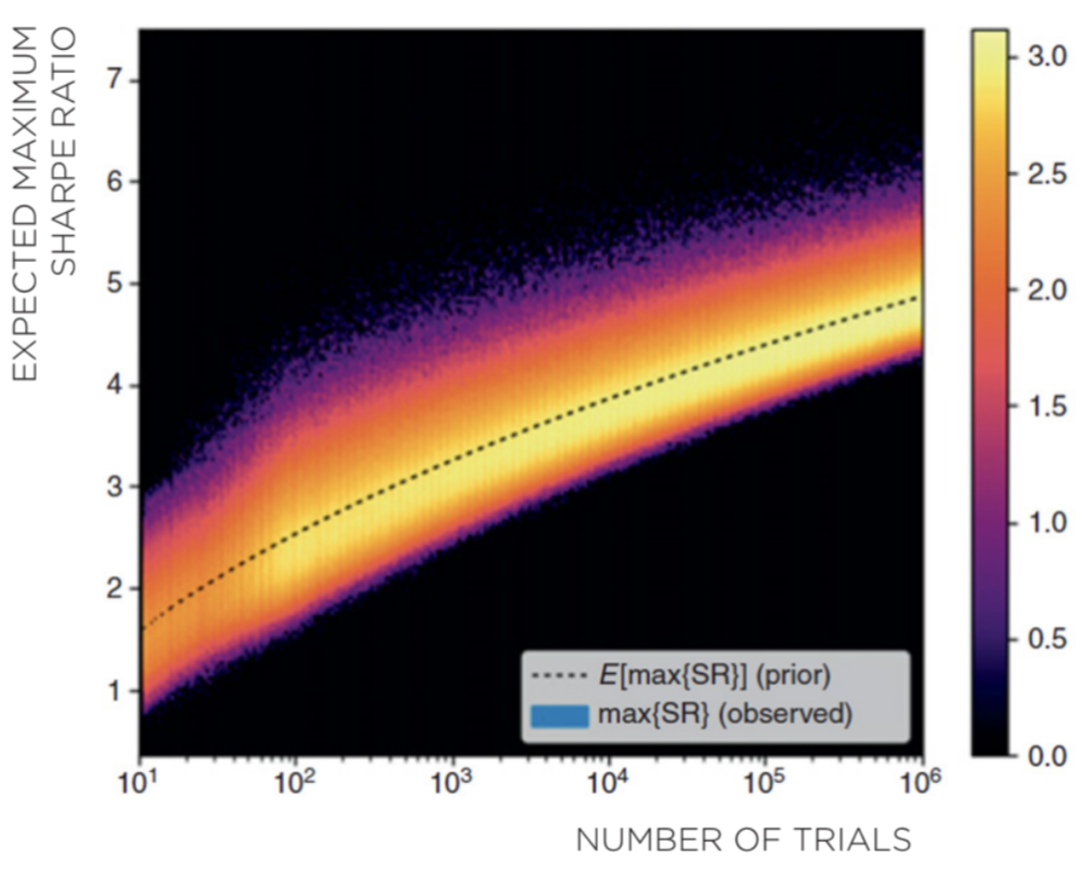
A famous example of this behavior is represented by the research conducted by Marcos Lopez De Prado – former head of Machine Learning at AQR – on the empirical distribution of the Sharpe ratios, as we can see from the following Exhibit. From the graph below – named provocatively “the most important plot in finance” – we can notice that after only 1,000 independent backtest trials, there is already a very high probability of experiencing a maximum Sharpe ratio above 3, when instead the real value of the strategy is null. This is why it takes extensive expertise and proper protocols to avoid identifying false-positive performing strategies.
Indeed, there are many reasons why a backtest can be flawed or biased and result in an abnormal Sharpe ratio.
Flaws in the Methodology
These flaws refer to the set of errors that stem out of an incorrect methodology for backtesting an investment strategy. They are very severe as they alter the structure of the simulations and therefore its overall validity.
For example, they occur when the analysis is performed exclusively at the in-sample level, meaning that there is not a subsequent analysis period that checks the consistency of the strategy on never seen observations – the so-called out-of-sample set. Indeed, without this step there would not be enough evidence to support the idea that the results obtained are not just the result of luck or data mining.
Model Overfitting
The practical consequence of backtest overfitting is the risk that a potential investment strategy will perform poorly when deployed in the real world.
Although this can happen for several reasons, the most common ones are represented by unjustified complexity and parameter tweaking. The first one is connected to the use of an over-complex model to describe a given investment strategy, resulting in extreme sensibility to different input data. The second one happens when the good results (in terms of performance) are artificially achieved by systematically searching for the model or the set of parameters that best fit the sample data thousands of times going back in history.
Data analysis biases
A backtest can be flawed also because of the low quality or incorrect use of data. Here, bias refers to the introduction of false or misleading information that causes estimates to be imprecise or systematically wrong.
Among this class, the most frequent are the ones connected to data quality, survivorship bias (i.e. exclusion of no-longer-existing data from the analysis sample), lookahead bias (i.e. including information that would not have been available during the period under analysis) and time-period bias (i.e. analysis results are largely attributable to the selection of the time window or its starting period).
The Forward-Looking Approach
Building on what we have seen until now, numerous insights have emerged from the analysis of portfolio optimization that can help us to better frame and understand the benefits associated with this technique.
First, we have understood the mechanism that leads some portfolios to be more efficient than others, that is, the role of diversification as a way to reduce the volatility without affecting the expected return. This is achieved by identifying and analysing the information contained in the three variables that define the underlying structure of financial markets: expected returns, volatilities and correlations.
We have focused on how portfolio optimization works in practice, highlighting its benefits as a way to efficiently select a portfolio according to an investor’s risk profile. Then we looked closely at the real meaning of efficiency, finding out not only that there is not a one-size-fits-all measure to capture this relation, but also that relying only on a simple efficiency maximization may not lead to what we initially expected.
Indeed, we understood that together with efficiency, the stability of our portfolio is an extremely important component that we must take into account in the optimization process. This has led us to focus on two additional features, namely the reliability of the process we use to determine the expected efficiency, and profitability, of a strategy together with the need for a dynamic approach to closely follow the gradual evolution of financial markets.
On the one hand, we have described which errors we must avoid while conducting research and where the potential sources of bias may lie.
On the other hand, we have seen that efficient frontiers evolve over time and so do the associated risk profiles of efficient portfolios.
When we put together all those insights we see more clearly the direction to follow to reap the benefits of this approach and add value to our investment decisions.
Indeed, what appears key to address this point is understanding that efficiency is the effect, rather than the cause of performance, and that a forward-looking approach is needed to build more robust portfolios.
Eventually, reframing the traditional portfolio optimization framework in these terms is essential to see through the complexity with a controlled and rational approach rooted in the application of the scientific method to the analysis of financial markets.
In this sense, transitioning from the traditional to the forward-looking aproach to portfolio optimization is how we can build portfolios that are stable, efficient and well-positioned to face the evolution of financial markets.
Look in the Windshield, Not in the Rearview Mirror
As we have seen, the idea behind portfolio optimization is a powerful one and we must handle it with great care and expertise to not fall prey to the many sources of bias that may alter the quality of our results.
During the years the initial framework laid down by Markowitz has received several improvements to address its restrictive assumptions. However, even though now we have better tools, performing portfolio optimization per se seems to be useless without taking into consideration its real-world application.
Eventually, instead of a one-size-fits-all solution, we should look at this process from a different perspective, as a systematic approach to navigate the complexity of financial markets and understand their underlying dynamics. As financial markets change constantly, what investors should look after is a forward-looking approach to build portfolios that are stable, efficient and well-positioned to face the evolution of financial markets.